UvA Data Science Center Seminar: Scalable Knowledge Discovery

Lab 42. Image source: https://campus.uva.nl/science-park/lab42/lab42.html
Scalable Knowledge Discovery
This blog post is derived from a seminar I gave at the University of Amsterdam Data Science Center.
Full seminar notebook with runnable code: https://github.com/erkankarabulut/DSC_seminar
git clone https://github.com/erkankarabulut/DSC_seminar.git
cd DSC_seminar
jupyter notebook knowledge_discovery_seminar.ipynb
Part 1: Knowledge Discovery Introduction
Knowledge discovery is described as nontrivial extraction of implicit, previously unknown, and potentially useful information from data (Frawley et al., 1992).
Our focus in this blog post is on a specific type of knowledge discovery, namely Association Rule Mining (ARM): finding co-occurrence patterns in tabular data (Agrawal et al., 1994).
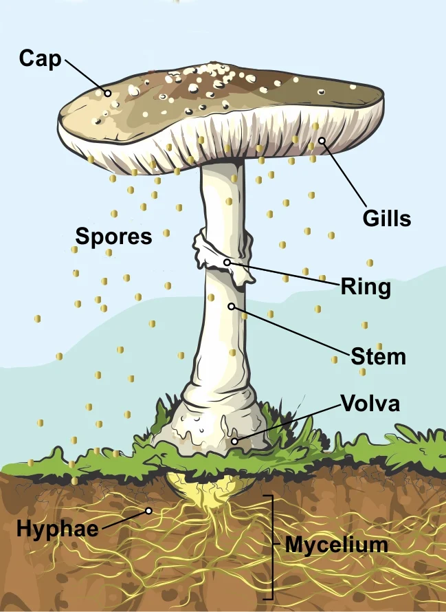
Consider a small mushroom dataset sample:
| cap-shape | cap-color | odor | habitat | poisonous |
|---|---|---|---|---|
| bell | brown | foul | woods | yes |
| convex | brown | none | woods | no |
| convex | brown | none | woods | no |
| convex | brown | none | woods | no |
| bell | red | foul | urban | yes |
| convex | brown | none | woods | no |
| flat | brown | almond | woods | no |
| convex | brown | none | woods | no |
Let’s extract some co-occurrence patterns from this data. What are some common characteristics of edible mushrooms?
Pattern P1: {cap-color=brown, habitat=woods, poisonous=no}
How often does this pattern occur in the data?
support(P1) = 6/8 = 75%. A good (high) number!
We can form association rules from this pattern, some of which are:
- A1:
{cap-color=brown} → {poisonous=no} - A2:
{habitat=woods} → {poisonous=no} - A3:
{cap-color=brown, habitat=woods} → {poisonous=no} - A4:
{cap-color=brown, poisonous=no} → {habitat=woods}
Note that a → (b ∧ c) is equivalent to (a → b) ∧ (a → c).
How accurate are they?
- confidence(A1) 6/7 = ~85%.
- confidence(A2) = 6/7 = ~85%.
- confidence(A3) = 6/6 = 100%.
- confidence(A4) = 6/6 = 100%.
Association Rule Mining (ARM): Find rules of the form
A → Cwheresupport(A → C) > min_support_thresholdandconfidence(A → C) > min_confidence_threshold(or any other quality metrics).
Do we just find high support and confidence rules then?
Imagine we set min_support_threshold = 50%.
Pattern P2: {odor=foul} → {poisonous=yes} (support=2/8=25%, confidence=100%)
A 100% confidence rule would be missed!
Observation High support rules can be good at explaining the trends in the data, while low support rules may refer to rare but critical patterns, anomalies, minority classes etc. The threshold should depend on the goal of knowledge discovery!
High confidence rules have to be interesting?
Let’s ask “which features actually affect poisoning risk?”
Pattern P3: {cap-color=brown} → {habitat=woods} (support=~85%, confidence=100%)
But … support({cap-color=brown}) = 85%. So any feature will imply {habitat=woods} anyways?
confidence({cap-shape=convex} → {habitat=woods})(confidence=100%)confidence({cap-shape=flat} → {habitat=woods})(confidence=100%)- …
So many not interesting rules (rule explosion problem) …
Rule explosion: Excessive number of rules that are expensive (computationally) to learn and hard to interpret.
Introduce another quality metric, association
strength (Zhang et al., 2009)
association_strength(A → C) = (confidence(A → C) - confidence(A’ → C)) / (max(confidence(A → C), confidence(A’ → C)), range [-1, 1]. -1: dissociation, 0: independence, 1: association.
association_strength({cap-shape=convex} → {habitat=woods}) = (1 - 0.66) / 1 = 0.33, barely interesting!
So this is it then, association strength is the answer?
association_strength({habitat=woods} → {cap-color=brown}) = 100%!
But …, support({habitat=woods}) = support({cap-color=brown}) = ~0.85. So the rule just says one common feature
implies another common feature.
Insight: There are no globally “good” patterns - you must define what matters for your task.
Part 2: Algorithmic Rule Mining
The most popular (and only) approach to mine rules from categorical datasets, until now …
Frequent Pattern-Growth (FP-Growth)
FP-Growth (Han et al., 2000) builds a compact tree structure ( FP-tree) to mine frequent patterns efficiently.
Example: Given transactions from our mushroom data (min_support = 3):
T1: {woods, brown, pink, no}
T2: {woods, brown, pink, no}
T3: {woods, brown, pink, no}
T4: {woods, brown, white, no}
T5: {woods, foul, buff, yes}
T6: {urban, foul, buff, yes}
Step 1: Count item frequencies → woods:6, brown:4, no:4, pink:3, foul:2, …
Step 2: Build FP-tree (ordered by frequency):
         root
          |
       woods:6
          |
       brown:4
        /   \
    pink:3  white:1
      |       |
     no:3    no:1
      |
   (foul:2, buff:2, yes:2 paths...)
Step 3: Mine patterns by traversing paths:
- Follow paths from leaves to root
- Generate frequent itemsets: {woods}, {brown}, {woods,brown}, {woods,brown,pink}, etc.
Step 4: Form rules and filter by confidence/support
Let’s load a mushroom dataset from the UCI ML repository, and run
FP-Growth with Mlxtend.
First, we install some required Python packages:
pip install ucimlrepo pandas mlxtend
import pandas as pd
from ucimlrepo import fetch_ucirepo

# load the mushroom dataset from ucimlrepo
mushroom = fetch_ucirepo(id=73)
mushroom = pd.concat([mushroom.data.features, mushroom.data.targets], axis=1)

print(f"Samples: {mushroom.shape[0]} | Features: {mushroom.shape[1]-1}")
print(mushroom[mushroom.columns[:5]].head())
import warnings
warnings.filterwarnings('ignore')

import time
from mlxtend.frequent_patterns import fpgrowth, association_rules
from mlxtend.preprocessing import TransactionEncoder

# one-hot encode the table
encoded_mushroom = [
        [f"{column}__{value}" for column, value in row.items()]
        for _, row in mushroom.iterrows()
]
te = TransactionEncoder()
te_ary = te.fit(encoded_mushroom).transform(encoded_mushroom)
encoded_mushroom = pd.DataFrame(te_ary, columns=te.columns_)

start_time = time.time()
frequent_itemsets = fpgrowth(encoded_mushroom, min_support=0.3, use_colnames=True, max_len=3)
rules_fp = association_rules(frequent_itemsets, metric="confidence", min_threshold=0.8)
fp_time = time.time() - start_time

print(f"Rules generated: {len(rules_fp)} (time: {fp_time:.2f}s)")
print(f"\nTop 5 rules by confidence:")
print(rules_fp.sort_values('confidence', ascending=False)[['antecedents', 'consequents', 'support', 'confidence', 'lift']].head())
Re-run the code with different min_support values: 0.2, 0.1, 0.05 …
Observation: Even for rules of size 3-items in a relatively small dataset (22 columns, 8K rows), mining is taking so long for relatively low support values. Traditional ARM methods are not scalable!
Part 3: Neurosymbolic Rule Mining - Aerial
Key idea
Instead of enumerating all itemsets, train an autoencoder to learn feature associations (Karabulut et al., NeSy Conference, 2025).
Autoencoders: a neural network architecture that is commonly used for representation learning, dimensionality reduction etc. (Vincent et al., 2008).
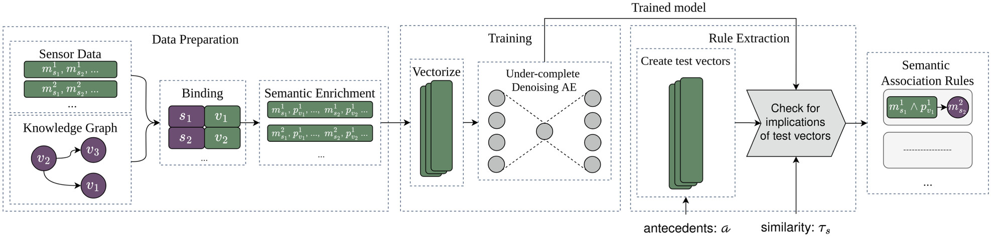
Pipeline:
- convert tabular data to one-hot encoded vectors
- train an Autoencoder to learn to reconstruct the table from a lower dimensional representation
- extract rules by exploiting the reconstruction ability of autoencoders (rules/patterns by reconstruction success)
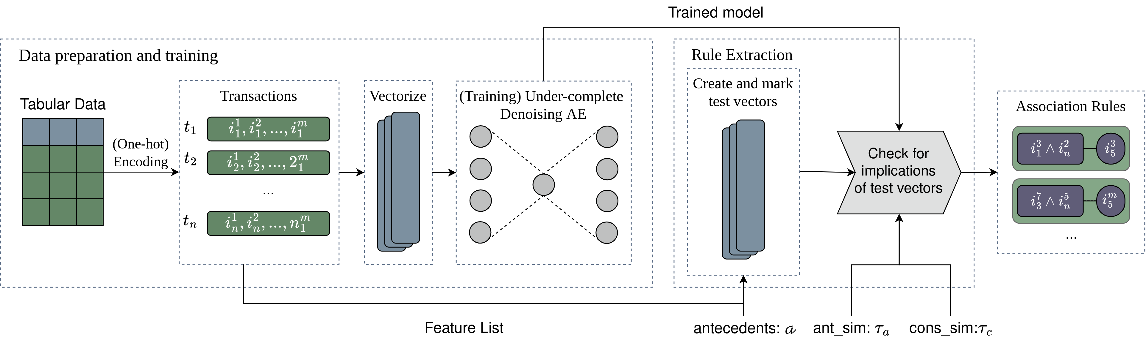
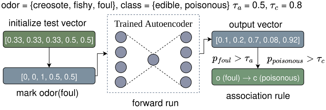
Rule extraction
Intuition: after training, given a partially constructed data point with marked features A and equal probabilities per class for the rest of the features, indicating no prior knowledge, if a set of features C are successfully reconstructed, then A → C.
Why it works?:
- By learning to reconstruct the data, autoencoders also learn feature associations.
- Successful reconstruction requires the knowledge of feature associations.
Benefits
- Capturing non-linear, more complex relations in the data than simply counting.
- Redundant patterns in the data do not help reconstruct the data, so they are eliminated (addressing the rule explosion issue).
- No longer need to ‘count’ co-occurrences. Significant improvement in execution time!
PyAerial: Python package for Aerial with many features: https://github.com/DiTEC-project/pyaerial
Software paper of PyAerial and benchmarking is at (Karabulut et al., SoftwareX Journal, 2025).
pip install pyaerial
# Set random seeds for reproducibility across all libraries
# This ensures consistent results when training neural networks and generating rules
import random
import numpy as np
import torch
import os

def set_seed(seed=42):
    random.seed(seed)
    np.random.seed(seed)
    torch.manual_seed(seed)
    torch.cuda.manual_seed_all(seed)
    # Make PyTorch operations deterministic
    torch.backends.cudnn.deterministic = True
    torch.backends.cudnn.benchmark = False
    # Set a fixed value for the hash seed
    os.environ['PYTHONHASHSEED'] = str(seed)
from aerial import model, rule_extraction
from ucimlrepo import fetch_ucirepo

set_seed()

# Train an autoencoder on the loaded table
trained_autoencoder = model.train(mushroom, batch_size=64)

# Extract association rules with quality metrics calculated automatically
result = rule_extraction.generate_rules(trained_autoencoder)

print(f"Overall statistics: {result['statistics']}\n")
print(f"Sample rule: {result['rules'][0]}")
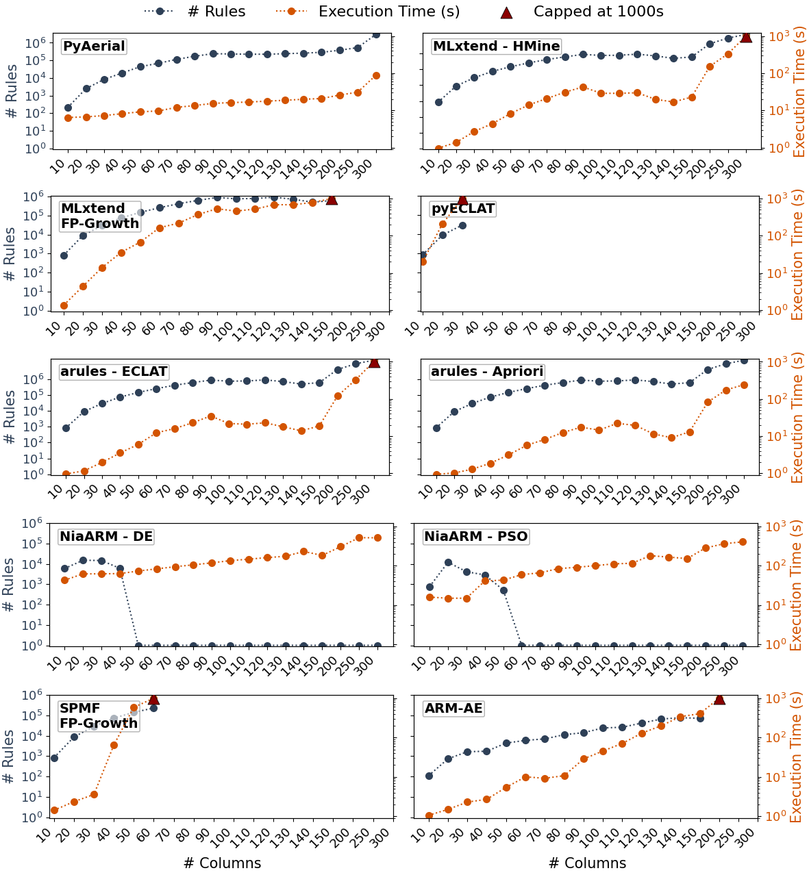
Observation: Simply eliminating the counting operation rule mining significantly sped up knowledge discovery!
PyAerial is 100s of times faster than other Python rule mining implementations! See our benchmarking paper for details.
Do we have control over the rules we learn?
Yes. Aerial parameters and architecture is easily controllable through PyAerial interfaces.
Experiment 1. Antecedent similarity threshold: lower values results in lower average support.
set_seed()

high_support_rules = rule_extraction.generate_rules(trained_autoencoder, ant_similarity=0.5)
print(f"High antecedent similarity: {high_support_rules['statistics']}\n")

low_support_rules = rule_extraction.generate_rules(trained_autoencoder, ant_similarity=0.2)
print(f"Low antecedent similarity: {low_support_rules['statistics']}\n")
Experiment 2. Consequent similarity threshold: higher values results in higher confidence rules.
set_seed()

high_confidence_rules = rule_extraction.generate_rules(trained_autoencoder, cons_similarity=0.8)
print(f"Low consequent similarity: {high_confidence_rules['statistics']}\n")

low_confidence_rules = rule_extraction.generate_rules(trained_autoencoder, cons_similarity=0.95)
print(f"High consequent similarity: {low_confidence_rules['statistics']}\n")
Experiment 3. Autoencoder compression (dimensionality reduction): more aggressive compression leads to smaller but higher-quality number of rules.
set_seed()

trained_autoencoder = model.train(mushroom, batch_size=64, layer_dims=[50])
low_compression_result = rule_extraction.generate_rules(trained_autoencoder)
print(f"Lower compression: {low_compression_result['statistics']}\n")

trained_autoencoder = model.train(mushroom, batch_size=64, layer_dims=[4])
high_compression_result = rule_extraction.generate_rules(trained_autoencoder)
print(f"Higher compression: {high_compression_result['statistics']}\n")
Observation: One fundamental issue in knowledge discovery is that users should already have a hypothesis in mind to get meaningful results by communicating this hypothesis to the algorithms and models, e.g., via setting proper criteria or thresholds. Data compression eases this process as it decides by itself what to preserve and what to discard!
Experiment 4. In deep learning, which is mostly done for predictive tasks, longer training results in overfitting. What does that mean for knowledge discovery?
set_seed()

trained_autoencoder = model.train(mushroom, batch_size=64, epochs=2)
shorter_training_result = rule_extraction.generate_rules(trained_autoencoder)
print(f"Shorter training: {shorter_training_result['statistics']}\n")

trained_autoencoder = model.train(mushroom, batch_size=64, epochs=10, patience=50, delta=1e-3)
longer_training_result = rule_extraction.generate_rules(trained_autoencoder)
print(f"Longer training: {longer_training_result['statistics']}\n")
Observation: Longer training in knowledge discovery means more rules with lower average quality!
What else can we do with PyAerial?
Rule learning with item constraints
Instead of exploring the entire search space for knowledge discovery, focus on specific features of interest.
set_seed()

trained_autoencoder = model.train(mushroom, batch_size=64)

# we can constrain rule generation on a feature level as well as on a class level
features = ["odor", "population", {"habitat": "woods"}]
result = rule_extraction.generate_rules(trained_autoencoder, features_of_interest=features)
print(f"ARM with item constraints: {result['statistics']}\n")
print('\n'.join(map(str, result["rules"][:3])))
Classification rules
Learn rules that have a certain class label on the consequent side. This can be used to “explain” class labels, as well as for interpretable decision-making in high-stakes scenarios. See our NeSy paper, Section 4.2.
set_seed()

trained_autoencoder = model.train(mushroom, batch_size=64)

# we can constrain rule generation on a feature level as well as on a class level
target = ["poisonous"]
result = rule_extraction.generate_rules(trained_autoencoder, target_classes=target)
print(f"Classification rules: {result['statistics']}\n")
print('\n'.join(map(str, result["rules"][:3])))
Classification rules can be integrated with algorithms that build rule-based classifiers, such as CORELS. See imodels for more details.
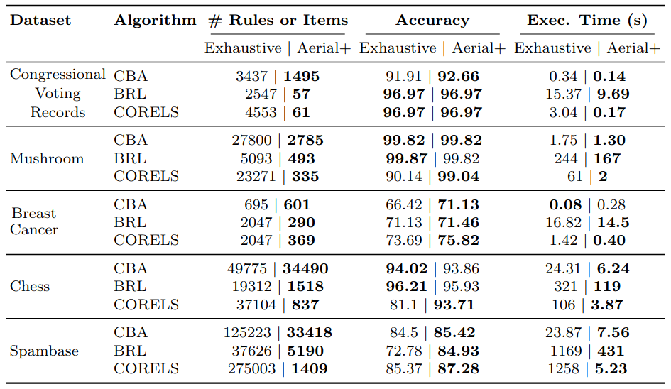
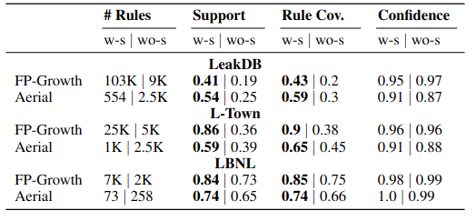
Empirical results: The smaller number of rules learned by Aerial leads to equal or higher accuracy in comparison to mining a significantly higher number of rules with algorithmic rule miners.
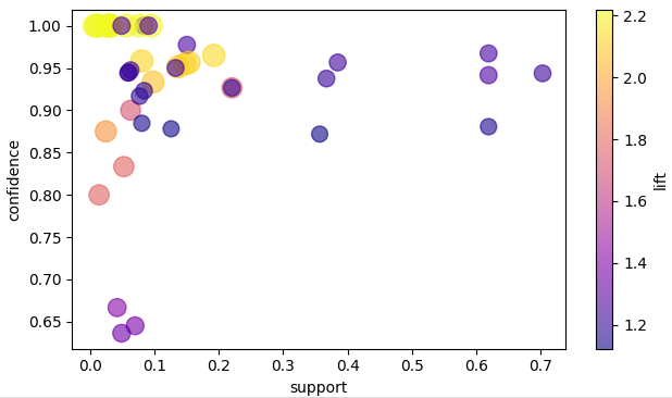
Visualizing rules
We can use existing rule visualization software to create nice visualizations. See our documentation: https://pyaerial.readthedocs.io/en/latest/user_guide.html#visualizing-association-rules.
Part 4: Advanced Topics in Knowledge Discovery
Research Question: What happens if there is not enough data to train on?
We can now utilize prior knowledge from tabular foundation models for knowledge discovery (Karabulut et al., ECAI Workshops, 2025)! This is not possible for classical algorithmic methods!
Boosting knowledge discovery with foundation tabular models
Strategy 1: use table embeddings from a tabular foundation model to initialize the weights of Aerial’s autoencoder.
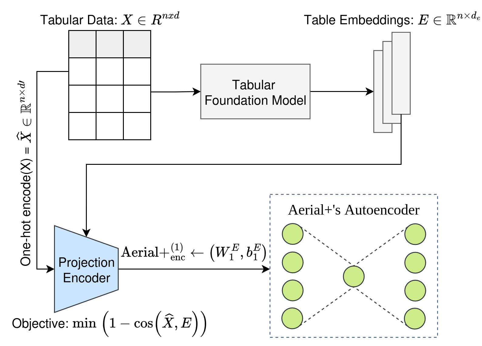
Strategy 2: use a projection encoder to align Aerial+ reconstructions with table embeddings from a tabular foundation model, jointly optimizing reconstruction and alignment losses for capturing table semantics better.
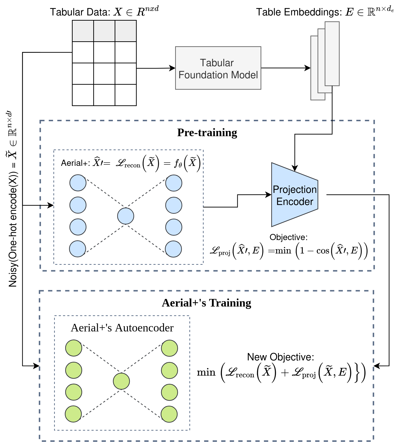
These strategies are evaluated on high-dimensional but small tabular datasets.
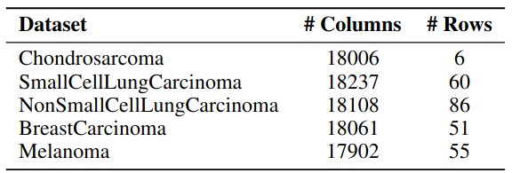
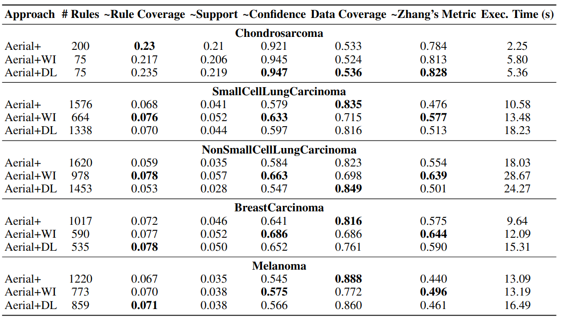
Empirical results: utilizing tabular foundation model embeddings led to an even smaller number of rules with higher quality. Using prior knowledge to boost knowledge discovery!
Research Question: Can we also include structured knowledge in the knowledge discovery process, e.g., knowledge graphs?
Yes. We can incorporate structured knowledge from a knowledge graph, e.g., giving more context to data, providing domain knowledge etc. (Karabulut et al., NAI Journal, 2025).
Below is a knowledge graph of a water distribution network.
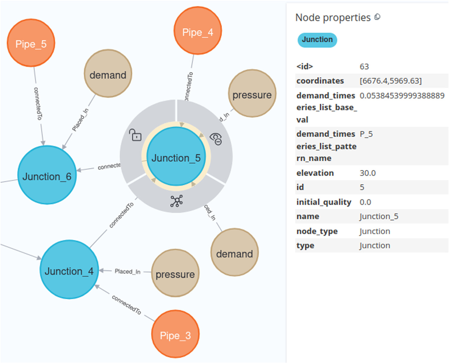
We can semantically enrich tabular data using a knowledge graph.
The same idea holds across many domains. E.g., in biomedicine, we know how certain proteins, genes and diseases interact. And we can make use of this knowledge during knowledge discovery!
Empirical results: Using structured knowledge during knowledge discovery leads to more generalizable patterns!
Rule without semantics: if sensor1 measures a value in range R, then sensor2 must measure a value in range R.
Rule with semantics: if a water flow sensor placed in a pipe P1 with diameter ≥ A1 measures a value in range R, then a water pressure sensor placed in a junction J1 connected to P1 measures a value in range R2.
Key takeaways
- Knowledge disovery is an unsupervised task, with no ground truth best patterns. It is all task-dependant.
- Neurosymbolic association rule mining is scalable, and more interpretable!
- PyAerial can help you discover various types of patterns in your data in a few lines of code.
- Prior knowledge from a foundation model can boost knowledge discovery.
- Structured knowledge can help learn more generalizable patterns in your data.
Future work
- Neurosymbolic rule mining has a plethora of applications: Anomaly/out-of-distribution detection, feature selection, classification, subgroup discovery and many more.
- What other prior/background knowledge can be utilized in knowledge discovery?
- More efficient ways of integrating prior/background knowledge is needed.
- PyAerial on numerical data, without pre-discretization.
- Can interpretable machine learning models compete with pure deep learning models, are we sacrifising accuracy for interpratability?
Resources
**Full seminar notebook with code: ** https://github.com/erkankarabulut/DSC_seminar
📄 **Aerial+ Paper: ** https://proceedings.mlr.press/v284/karabulut25a.html
🐍 PyAerial Library: https://github.com/DiTEC-project/pyaerial
📦 PyAerial on PyPI: https://pypi.org/project/pyaerial/
📚 PyAerial Documentation: https://pyaerial.readthedocs.io/
Collaboration: For discussions on neurosymbolic knowledge discovery and interpretable inference, reach out at e.karabulut@uva.nl